Summary
This analysis is an exercise in reproducibility and literate programming with ecological data. This page is produced as a distill article (https://rstudio.github.io/distill/) created from an R Markdown file in R Studio (R version 4.1.2). The goal of this document is to highlight best practices in reproducible research including using literate programming with inline coding to accompany code chunks, resulting in a dynamic document where the analysis & accompanying text update each time the API returns newly entered data.
In this example, the occurrence of the Sierra newt (Taricha sierrae) is inferred from occurrence records accessed from the Global Biodiversity Information Facility (GBIF, https://www.gbif.org/).
Introduction
Appropriate conservation policy requires thoughtful actions driven by precise information. Further, insight into the ecology of a species can be inferred through the careful use of spatially-accurate occurrence data. This document explores the distribution of the Sierra newt (Taricha sierrae), a California endemic caudate that inhabits the Sierra Nevada Mountain Range along the east-central margin of the state. Four species are currently recognized in the genus Taricha, with T. sierrae having been elevated to full species status in 2007 (Kuchta 2007). This analysis will include observations classified under the currently accepted nomenclature, Taricha sierrae, as well as the synonyms Taricha torosa sierrae & Triturus sierrae.
Finally, the Sierra newt is listed as ‘Least Concern’ by the International Union for Conservation of Nature (IUCN 2021) and is not listed as a ‘Species of Special Concern’ by the state of California (CNDDB 2022; Thomson 2016), making it an ideal candidate for an exercise in best practices for georeferencing sensitive species (Category 4, table 6: Chapman 2020). However, it is important to note that two out of the four species in the genus are listed as ‘Species of Special Concern’ in California: the Red-bellied newt (T. rivularis) and the southern populations of the Coast Range newt (T. torosa) (CNDDB 2022). Therefore, occurrence data for these species will not be included.
Setup
Load Packages
Obtain Occurrence Records
The Global Biodiversity Information Facility (GBIF) API is accessed through the gbif function in the dismo package (https://github.com/rspatial/dismo).
sn_gbif <- dismo::gbif("Taricha", "sierrae", download = T, geo = T)
The gbif function returned 1230 observations of the Sierra newt from the GBIF API.
Aforementioned in the Introduction, this analysis will include records of all synonyms for the Sierra newt. The API returns records listed under 3 names: Taricha sierrae (Twitty, 1942), Taricha torosa sierrae (Twitty, 1942), Triturus sierrae Twitty, 1942.
sn_names <- table(sn_gbif$scientificName)
knitr::kable(sn_names, col.names = c("synonym", "frequency"))
| synonym | frequency |
|---|---|
| Taricha sierrae (Twitty, 1942) | 747 |
| Taricha torosa sierrae (Twitty, 1942) | 477 |
| Triturus sierrae Twitty, 1942 | 6 |
Exploratory Data Analysis
To begin initial exploratory data analysis, we can start by exploring some temporal aspects of the data, including month & year of occurrence record.
Temporal
Month of occurrencesn_gbif %>%
ggplot(aes(x = factor(month)))+
geom_histogram(fill = '#1200b3', stat = "count")+
labs(x = "month", y = "count",
title = "Histogram of observation month")+
scale_x_discrete(breaks = c(1:12), limits = factor(c(1: 12)))+
theme_bw()+
theme(panel.grid.major = element_blank(),
panel.grid.minor = element_blank())
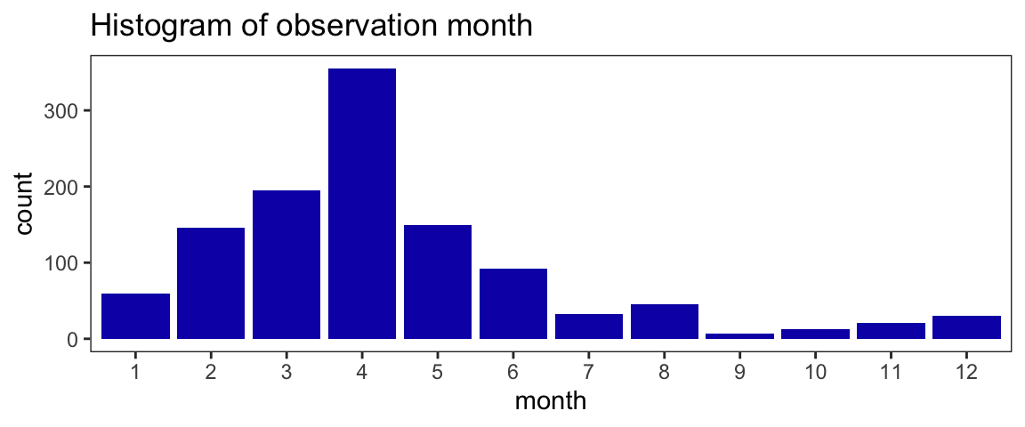
Observations of Sierra newt are not uniformly distributed throughout the year in the data. This is unsurprising, as many species are more conspicuous at certain times of the year, especially species with a seasonal migration such as the Sierra newt. The distribution peak in the months corresponding to spring in the northern hemisphere suggests most observations occur during breeding season for the Sierra newt, while individuals are migrating to or already at bodies of water for courtship & egg laying (Vance 2000).
Year of recordsn_gbif %>%
ggplot(aes(x = year))+
geom_histogram(bins = 20, fill = '#1200b3')+
labs(x = "year", y = "count",
title = "Histogram of year of observation")+
theme_bw()+
theme(panel.grid.major = element_blank(),
panel.grid.minor = element_blank())
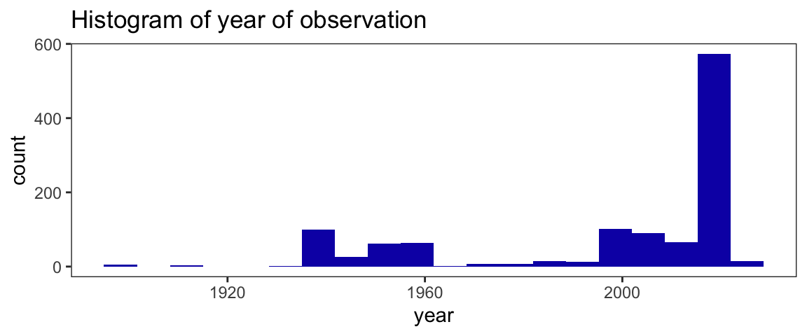
Data for year of observation are heavily left-skewed. More than 50% of records have occurred since 2016. The earliest observation was recorded in 1895, while the most recent observation is from 2022. The 79 records without year data (NA’s) will be filtered out later in the analysis.
Spatial
Elevation
For a species distributed over a mountain range, such as the Sierra newt, elevation may be a key niche component. Elevation data for each record are included in both the elevaiton and verbatimElevation columns in the data.
Of the total 1230 records returned by the GBIF API, 243 contain elevation data with the observation.
sn_elev_bor <- sn_gbif %>% dplyr::select(elevation, basisOfRecord) %>%
          mutate(with_elev = !is.na(sn_gbif$elevation)) %>%
          group_by(basisOfRecord, with_elev) %>%
          summarise(n = n()) %>%
          mutate(percent = round(n / sum(n) * 100, 2))
knitr::kable(sn_elev_bor, col.names =
                       c("type of record", "elevation_data?", "frequency", "percent"))
| type of record | elevation_data? | frequency | percent |
|---|---|---|---|
| HUMAN_OBSERVATION | FALSE | 651 | 100.00 |
| PRESERVED_SPECIMEN | FALSE | 336 | 58.03 |
| PRESERVED_SPECIMEN | TRUE | 243 | 41.97 |
100 percent of human observation records and 58 percent of preserved specimens lack elevation data. 42 percent of preserved specimen records contain elevation data.
Verbatim elevation
Similarly, 212 of the total 1230 records contain elevation data in the ‘verbatim elevation’ column.
sn_elev_verb_bor <- sn_gbif %>% dplyr::select(verbatimElevation, basisOfRecord) %>%
          mutate(with_elev_verb = !is.na(sn_gbif$verbatimElevation)) %>%
          group_by(basisOfRecord, with_elev_verb) %>%
          summarise(n = n()) %>%
          mutate(percent = round(n / sum(n) * 100, 2))
knitr::kable(sn_elev_verb_bor, col.names =
                       c("type of record", "elevation_data?", "frequency", "percent"))
| type of record | elevation_data? | frequency | percent |
|---|---|---|---|
| HUMAN_OBSERVATION | FALSE | 651 | 100.00 |
| PRESERVED_SPECIMEN | FALSE | 367 | 63.39 |
| PRESERVED_SPECIMEN | TRUE | 212 | 36.61 |
100 percent of human observation records and 63 percent of preserved specimen records lack elevation (verbatim) data. This is compared to 37 percent of preserved specimen records containing elevation data in the verbatim elevation column.
Coordinate uncertainty
To better understand the spatial data, we can examine the levels of accuracy in the coordinates.
sn_gbif %>%
          ggplot(aes(x = coordinateUncertaintyInMeters))+
          geom_histogram(bins = 20, fill = '#1200b3')+
          labs(x = "Coordinate uncertainty (meters)", y = "count",
               title = "Histogram of coordinate uncertainty")+
          theme_bw()+
          theme(panel.grid.major = element_blank(),
                panel.grid.minor = element_blank())
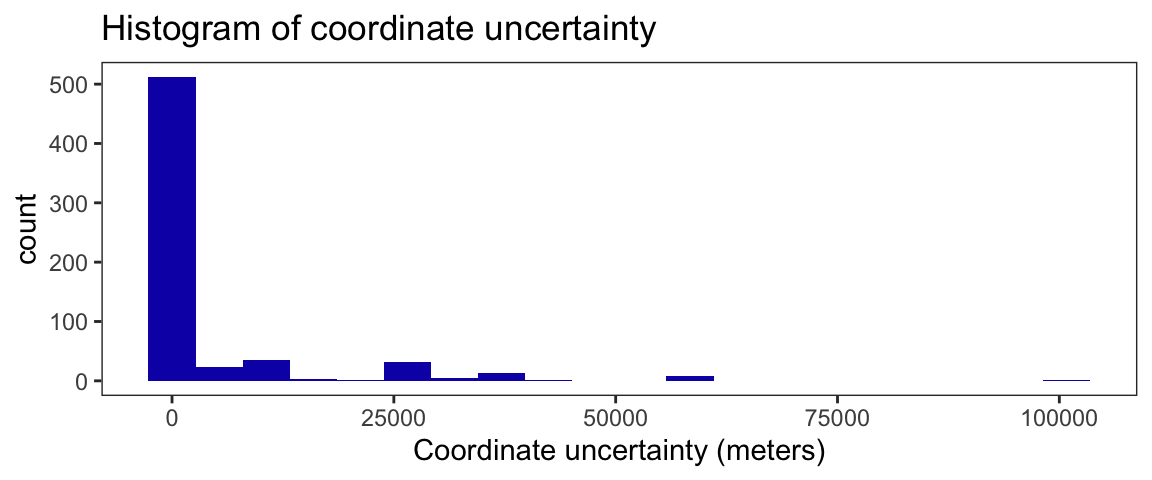
summary(sn_gbif$coordinateUncertaintyInMeters)
     Min.   1st Qu.    Median      Mean   3rd Qu.      Max.      NA's
     1.00     13.25    190.00   4489.55   1807.00 100838.00       596
Data for coordinate uncertainty are right skewed. The median uncertainty of coordinates is 190 meters. The minimum uncertainty was 1 meter, while the maximum uncertainty is 100838 meters.
Depending on the type of modeling to be undertaken, observations may be subsequently filtered to exclude records exceeding an acceptable level of coordinate uncertainty. One way of determining this threshold is by the spatial resolution (cell size) of the raster files depending on the scale of the specific analyses.
How does coordinate uncertainty of observations change with time?sn_gbif %>%
dplyr::select(coordinateUncertaintyInMeters, year) %>%
drop_na() %>%
ggplot(aes(x = year, y = log(coordinateUncertaintyInMeters))) +
geom_point(aes(color = coordinateUncertaintyInMeters),
alpha = 0.7,
size = 1.2)+
scale_colour_gradient(low = "blue", high = "red")+
labs(title = "Coordinate Uncertainty (Log) & Year of Observation",
x = "year", y = "Log coordinate uncertainty (meters)")+
theme_minimal()+
theme(legend.position="none")
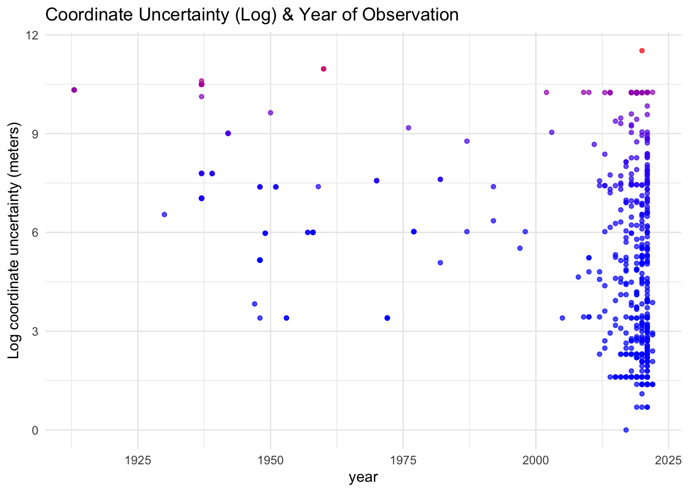
Figure 1: Points are colored as a gradient scale for coordinate uncertainty (log).
Because the data for observation year are heavily left-skewed, ie., there are substantially more observations recorded from recent years rather than earlier years, these data may not provide an accurate representation of any true relationship between time (year) & coordinate uncertainty (fig 1). While it may be tempting to fit a linear model, these data do not meet the assumption of normality for a linear regression, as these data are not normally distributed. Even without fitting a linear regression however, it is apparent that uncertainty varies largely, even in recent years. For example, the record containing the coordinates with the largest uncertainty is from 2020.
Further, while technological capabilities undoubtedly increase with time, eg., the arrival of GPS and subsequent use in citizen science applications for recording species occurrences, these data may come from a number of sources that may not relate to how precise the coordinates are recorded. In some instances, variation in coordinate uncertainty may simply be an artifact of how and where the measurement is taken (Chapman and Wieczorek 2020), for example diminished GPS accuracy beneath a dense canopy when recording an observation of a forest dwelling species. Moreover, deliberate uncertainty is frequently added to obscure spatial information, especially for the protection of species of concern (Chapman 2020). Therefore, the next phase of EDA should explore how these data were collected.
Source of Record
An important step in exploratory data analysis is to understand the source of the data. For certain analyses, it may be important to use only records collected through a specific means. To explore the source of these records, we can calculate some basic summary statistics for the “type of record,” basisofRecord column, to see how the data were collected.
sn_bor <- sn_gbif %>% group_by(basisOfRecord) %>%
          summarise(n = n()) %>%
  mutate(percent = round(n / sum(n) * 100, 2))

knitr::kable(sn_bor, col.names = c("type of record", "frequency", "percent"))
| type of record | frequency | percent |
|---|---|---|
| HUMAN_OBSERVATION | 651 | 52.93 |
| PRESERVED_SPECIMEN | 579 | 47.07 |
These data contain 651 records from human observations (eg., INaturalist records) & 579 records from preserved specimens from 16 institutions. For visualizing occurrence records, coordinates from both sources of data will be used for mapping.
Data Processing
For initial visualization of the spatial data, only simple data cleaning will be necessary. The first phase will be filtering out missing data.
Complete cases
Incomplete observations (records without data pertaining to name, year, coordinates & coordinate uncertainty) are removed from analysis. Data with missing elevation values are included for now, as elevation values for each observation can be calculated later in the modeling phase.
Clean coordinates
Coordinates for Sierra newt occurrences will be assessed for spatial outliers with the clean_coordinates function from the CoordinateCleaner package (https://github.com/ropensci/CoordinateCleaner).
sn <- clean_coordinates(x = sn,
                              lon = "lon",
                              lat = "lat",
                              species = "scientificName",
                              value = "clean")
OGR data source with driver: ESRI Shapefile
Source: "/private/var/folders/xm/gf1fm0154f72vtcv0mt_vvb80000gn/T/RtmpkphCa5", layer: "ne_50m_land"
with 1420 features
It has 3 fields
Integer64 fields read as strings:  scalerank
Vizualizing Spatial Data
Now that the data have completed some initial processing, mapping the coordinates can provide a better understanding of the distribution of this species.
To plot the occurrence records, the lon & lat columns in the data frame will be used as coordinates to convert to an sf object. For viewing the coordinates, the coordinate reference system (CRS) will be set to ‘EPSG::4326,’ as the data (column geodeticDatum) are of the type ‘WGS84.’
A great tutorial for georeferencing coordinates in R by Floris Vanderhaeghe: https://inbo.github.io/tutorials/tutorials/spatial_crs_coding/
Variation in Coordinate Data
To visualize occurrence records, we can map them with as sf using geom_sf with ggplot2.
sn_cu_yr <- sn %>% dplyr::select(lon, lat, year, coordinateUncertaintyInMeters) %>%
          st_as_sf(coords = c("lon", "lat"), crs = 4326)
ryr <- range(sn$year)

ggplot()+
          geom_sf(data = ca)+
          geom_sf(data = sn_cu_yr, aes(size = coordinateUncertaintyInMeters, col = year),
                  alpha = 0.5)+
          labs(title = "Map of GBIF occurrence records for the Sierra newt",
               subtitle = "Records by year of observation & coordinates uncertainty (meters)",
               x = "longitude", y = "latitude",
               color = "observation year", size = "coordinate uncertainty (m)")+
          theme_bw()+
          scale_size_binned(breaks = c(0, 10, 100, 1000, 10000, 10e6))+
          scale_colour_gradient2(low = "red", high = "blue",
                                 midpoint = mean(ryr), mid = "purple",
                                 limits = c(1930, 2030),
                                 breaks = c(1930, 1975, 2022))+
          guides(size = guide_bins(show.limits = TRUE))+
          coord_sf(crs = st_crs(4326),
                   xlim = c(-122.5, -118.5), ylim = c(36, 41.25))
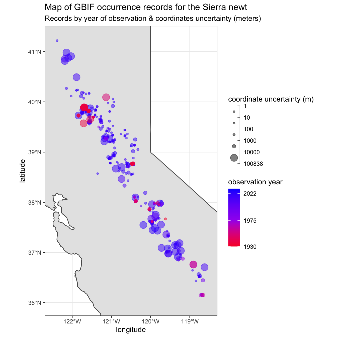
Figure 2: Map corresponding to central California with occurrence records of the Sierra newt, where point size is scaled to uncertainty of coordinates (meters) and point color as a gradient of record year.
Occurrence records appear to be distributed independently with respect to coordinate uncertainty & year of observation (fig 2). If a strong correlation existed between coordinate pairs (lon/lat) and observation year, red and blue points would not show substantial overlap. Additionally, there is a considerable number of intermediate (towards purple) points represented. Likewise, if a correlation existed between coordinates and coordinate uncertainty, large and small radius points (ie., coordinates with small and large uncertainties) would not regularly co-occur across the map. As a result, there appears to be significant mixing of point bin sizes (small through large) and point colors (blue through red) spread fairly consistently throughout the distribution.
Exploring Environmental Covariates
As above, we will begin by converting the lon & lat coordinates to sf objects a CRS.
Calculating elevation
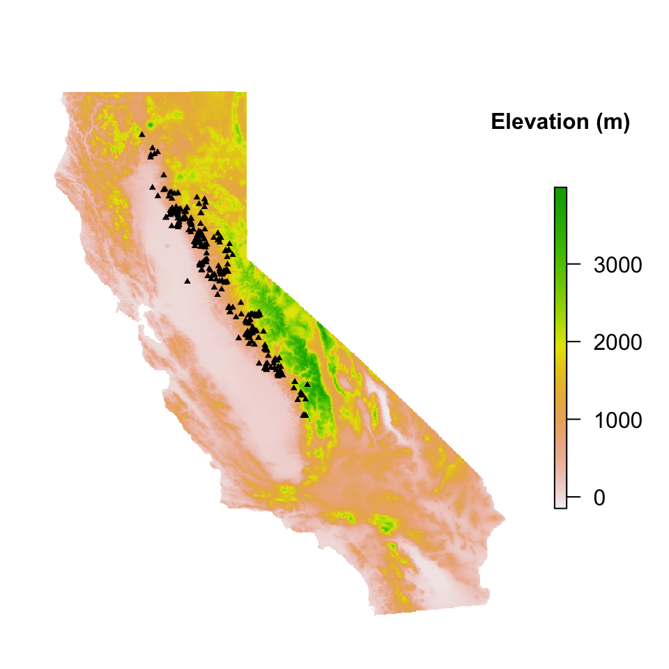
Elevation data can be calculated from the get_elev_raster function in the elevatr package. Note however that elevation values for each observation record will not be extracted from the elevation raster layer for modeling until more detailed cleaning of spatial information (including coordinates & filtering coordinate uncertainty). For this example, elevation will only be calculated for visualization and not to infer for each observation point.
# calculate elevation
elev <- elevatr::get_elev_raster(ca, z = 6)
# create CA extent
ca_extent <- extent(x = c(-125,-113, 32.25, 42.5))
# crop to CA extent
ca_elev <- crop(elev, ca_extent)
# mask to CA polygon
ca_crop_elev <- raster::mask(ca_elev, ca)

par(mar = c(0, 1, 1, 0))
plot(ca_crop_elev, axes = FALSE, box = FALSE, legend.args = list(text = 'Elevation (m)',
                                                             side = 3, font = 2,
                                                             line = 2, cex = 1))
points(sn_coords, pch = 17, cex = 0.5)
Mapview
This can be further explored using the interactive mapView function from the mapview package by plotting the elevation raster & including the spatial points as an sf object.
# interactive coordinate view
mapView(ca_crop_elev) + sn_coords_sf
The mapView function is useful as we can ensure our raster layers are projected appropriately and align with our data. Mapping occurrence data over an interactive map also allows us to explore any potential outliers or errors, such as observations located near urban Sacramento & Chico, CA. These records are discussed in detail below and addressed prior to any modeling.
Calculating slope, aspect, & hillshade
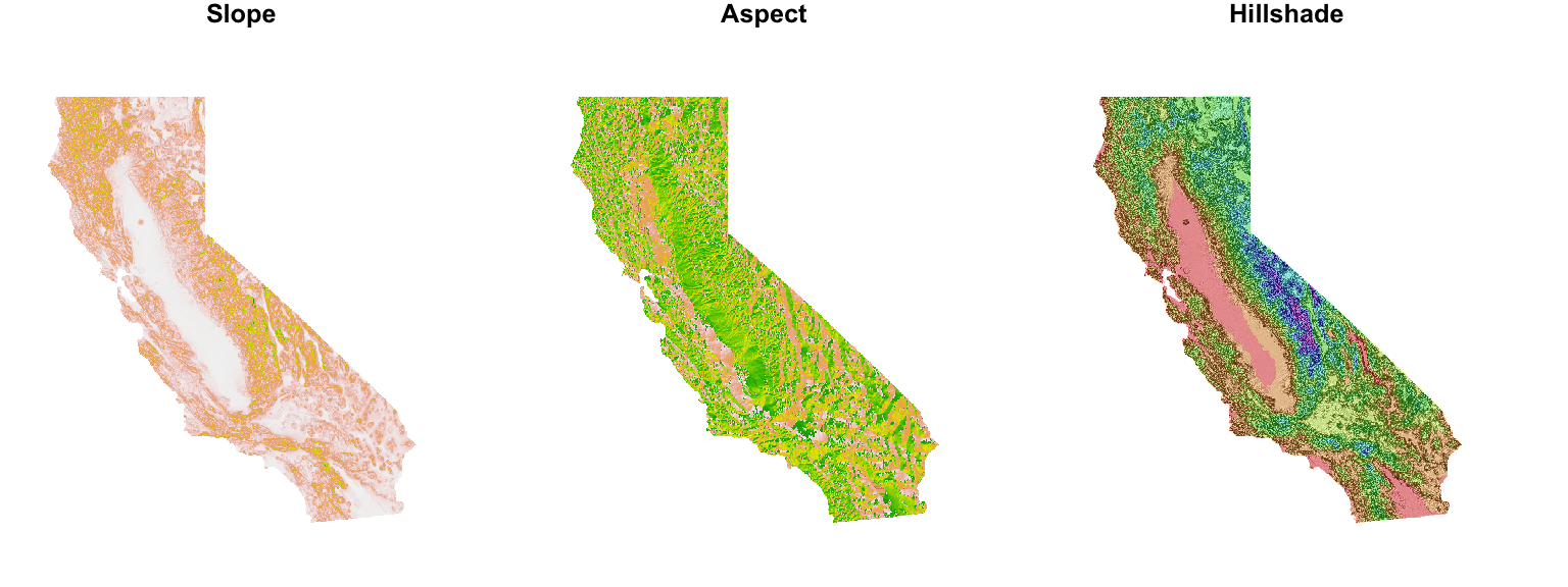
Having computed the elevation raster, the raster & terra packages can be used to calculate raster layers for slope, aspect & hillshade. Like elevation, these layers can also be used later in the modeling phase of the analysis if deemed of ecological significance for the species.
ca_slope <- terra::terrain(ca_crop_elev, opt = 'slope', unit = 'degrees')

ca_aspect <- terra::terrain(ca_crop_elev, opt = 'aspect', unit = 'degrees')

hill_shade <- raster::hillShade(ca_slope, ca_aspect)
#hill_shade = terra::shade(slope = ca_slope, aspect = ca_aspect, angle = 45, direction = 0)

par(mar = c(0.1, 1, 1, 1), mfrow=c(1, 3))
plot(ca_slope, main = "Slope", axes = FALSE, box = FALSE, legend = FALSE)
plot(ca_aspect, main = "Aspect", axes = FALSE, box = FALSE, legend = FALSE)
plot(hill_shade, col = grey(0:100/100), legend = FALSE, main = "Hillshade", axes = FALSE, box = FALSE)
plot(ca_crop_elev, col = rainbow(10, alpha = 0.35), add = TRUE, legend = FALSE)
3D plot with Rayshader
For an intuitive view of the occurrence of T. sierrae, the Rayshader package (https://www.rayshader.com/) can provide an interesting 3D visualization of the spatial distribution overlay with the occurrence records from the render_points function.
ca_elev_mat <- raster_to_matrix(ca_crop_elev)

# create texture palette
ca_texture <- create_texture(
          '#fceed2',
          '#000000',
          '#6b6250',
          '#362b16',
          '#73513d',
          cornercolors = '#111111')

#create shadows
ca_shadow = ray_shade(ca_elev_mat, zscale = 5, lambert = FALSE)
ca_ambshade = ambient_shade(ca_elev_mat, zscale = 5)

ca_elev_mat %>%
          sphere_shade(zscale = 5, texture = ca_texture) %>%
          add_shadow(ca_shadow, 0.5) %>%
          add_shadow(ca_ambshade, 0.5) %>%
          plot_3d(ca_elev_mat, zscale = 90,
                  baseshape = 'rectangle',
                  shadow_darkness = 0.7,
                  fov = 100, theta = -70, phi = .4,
                  windowsize = c(1000, 800), zoom = .7)
render_points(extent = attr(ca_crop_elev,"extent"), heightmap = ca_elev_mat,
              lat = sn_coords$lat, long = sn_coords$lon,
              zscale = 50, color = "cyan1", offset = 0, size = 5)
render_camera(theta = 0, phi = 90, zoom = .3, fov = 110)
render_snapshot()
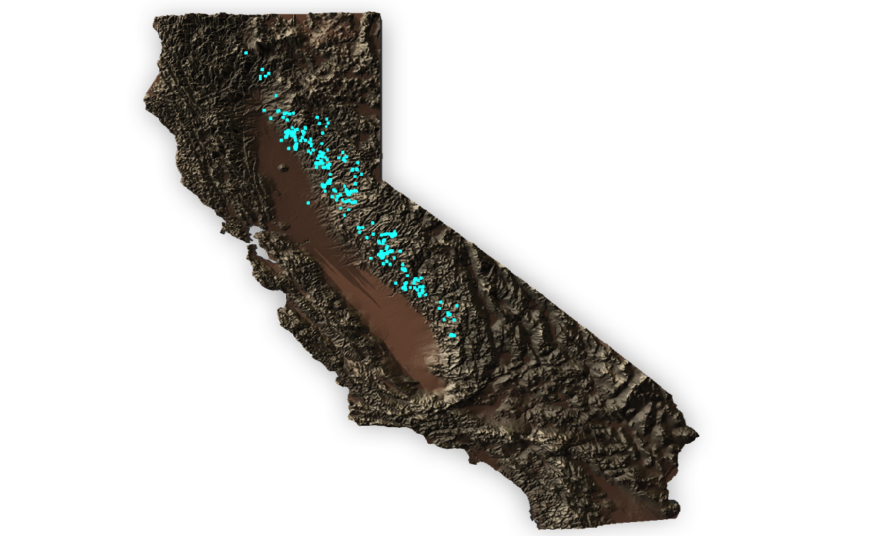
Figure 3: Rayshader 3D plot of California with occurrence points in cyan.
To better visualize the occurrence data in relation to elevation, we can modify the view:
ca_elev_mat %>%
          sphere_shade(zscale = 5, texture = ca_texture) %>%
          add_shadow(ca_shadow, 0.5) %>%
          add_shadow(ca_ambshade, 0.5) %>%
          plot_3d(ca_elev_mat, zscale = 90,
                  baseshape = 'rectangle',
                  shadow_darkness = 0.7,
                  windowsize = c(width = 1000, height = 1000), zoom = .7)
render_points(extent = attr(ca_crop_elev,"extent"), heightmap = ca_elev_mat,
              lat = sn_coords$lat, long = sn_coords$lon,
              zscale = 50, color = "cyan1", offset = 0, size = 5)
render_camera(theta = -105, phi = 25, zoom = .3, fov = 80)
render_snapshot()
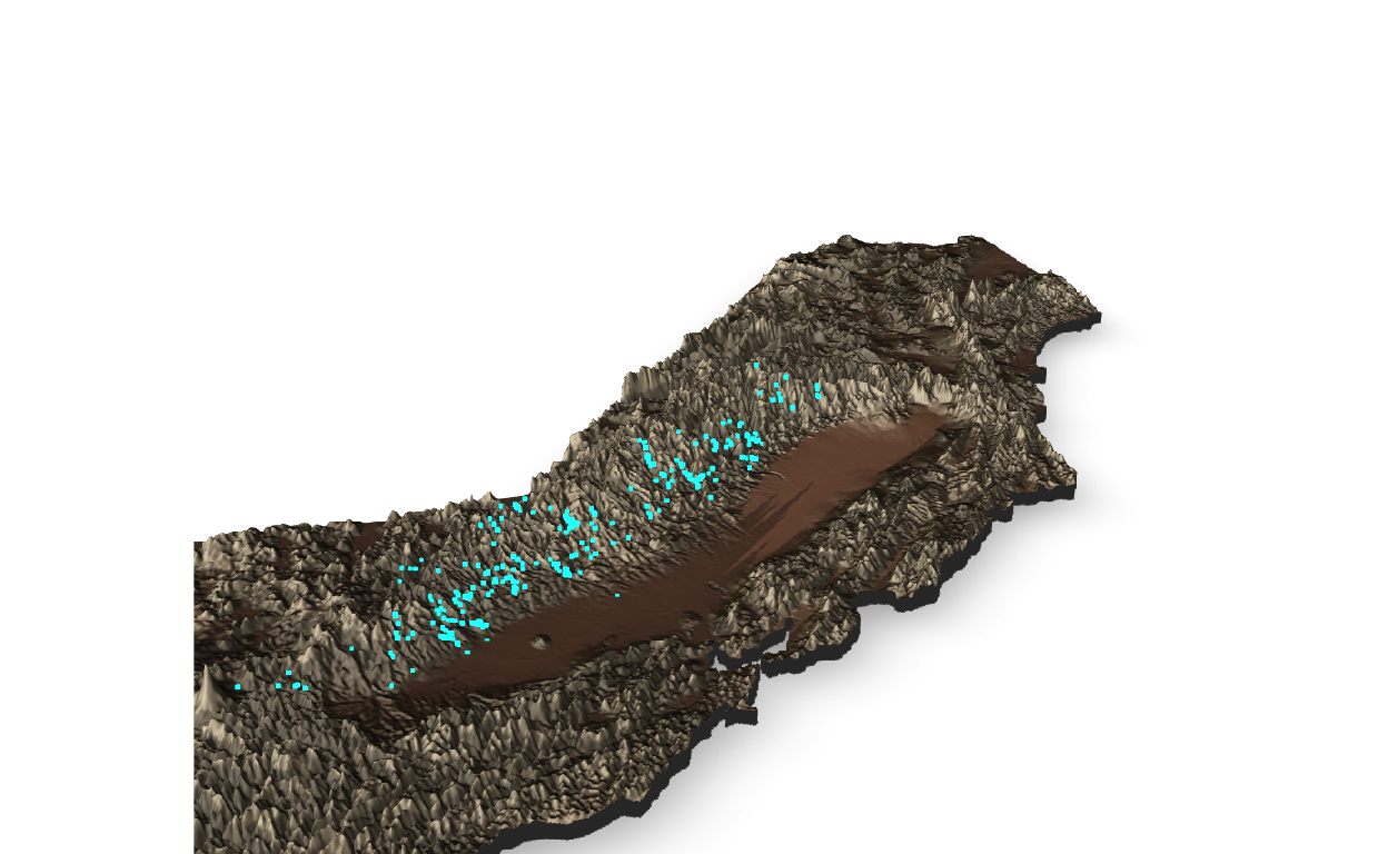
Figure 4: Rayshader 3D plot of California from a different rotation & lower angle.
Final Thoughts
Ecology
The 3D map created by the Rayshader package highlights the potential importance of elevation as a niche dimension for the Sierra newt. While some observations occur towards lower elevations, especially adjacent the Central Valley (see Spatial outliers & erroneous data chapter below), the majority of individual occurrences appear to be at elevations well above sea level within the Sierra Nevada Mountain Range (elevations for each observation will be extracted from the elevation raster and cross-checked prior to modeling).
So far, these occurrence records appear consistent with the ecology of T. sierrae, which are documented occurring up to about 2000 meters above sea level (Stebbins and McGinnis 2012). Like many other amphibians occurring in montane habitats, higher elevations may encompass key niche dimensions for the Sierra newt. Environmental variables, such as temperature & moisture availability, likely limit the distribution of amphibians. Desiccation may act as a mechanistic constraint on the availability of habitats to many high-elevation amphibians, inhibiting expansion into more arid environments at lower elevations. Further, the need for available breeding habitat, either as flowing streams or standing pools, would be restrictive on the range of this species. Distribution modeling, such as correlative or mechanistic approaches, may provide further insight into these factors.
Spatial outliers & erroneous data
Before modeling observation records, a deeper exploration of the data are required to ensure any inaccuracies are properly addressed. While the Clean Coordinates package helps in this area, it is crucial to parse records and flag any potential outliers. This includes, when an option, having a better look at the original record. Below are some examples of flagged records from this dataset.
https://www.inaturalist.org/observations/86987010 - One observation of interest is a record from a residence, adjacent to the American River at ~16.5 meters above sea level, in suburban Sacramento, California. The source of this record is an INaturalist observation from Jul 14, 2021. It may be appropriate to model these data by comparing model outputs from both including & excluding this observation. Because this species is known to be found down to sea level, it may be worth modeling both including & excluding this observation.
https://www.inaturalist.org/observations/71686701 - The record maps to the center of Chico, CA and has an accuracy of ~14.5km, according to the INaturalist observation. As a result, it is unlikely that this observation would be of much use in any spatial modeling due to such low accuracy and subsequently should be removed prior to analyses.
Next steps
Now that the initial phase of data exploration has concluded, the data can next be prepared for use in various modeling scenarios to answer a variety of ecological questions. For example, using the elevation raster layer calculated previously as one of the ecologically-significant environmental covariates for a correlative approach to modeling the distribution of the species.